Total Emissions
Contents
Total Emissions#
Exploring the functionality of NEMED to extract regional total emissions and corresponding emission intensities
Data Extraction#
Import Packages#
Show code cell content
import nemed
from nemed.downloader import download_aemo_cdeii_summary, download_unit_dispatch
from nemed.process import aggregate_data_by

# To generate plots shown
import pandas as pd
import numpy as np
import plotly.graph_objects as go
import plotly.express as px
from plotly.subplots import make_subplots

# Open plot in browser (optional)
import plotly.io as pio
pio.renderers.default = "browser"
Processing Emissions Data#
Total regional emissions and the regional emissions intensities can be extracted using get_total_emissions. The following inputs must be specified:
start_timedefine the start of the historical period to collect data for. Must be in the format: “yyyy/mm/dd HH:MM”end_timedefine the end of the historical period to collect data for. Must be in the format: “yyyy/mm/dd HH:MM”cachespecify the local file directory to temporarily store downloaded files
Optionally, you can also pass the arguments:
filter_regionsspecify a list of NEM regions to collect data for. If this is not specified, data is collected for all NEM regions. Must be a list of strings, e.g. [‘NSW1’,’VIC1’]byspecifys the time resolution to which the data is aggregated. Noting that raw (unaggregated) data is in 5-minute increments which can be obtained by setting this parameter to ‘interval’ or None.generation_sent_outif set true, auxiliary load factors are considered in the calculation of emissions (as per the CDEII method).assume_energy_rampif set true, a linear ramp assumption is used to calculate energy generation (MWh). Setting this false will significantly improve computation time but yield less accurate results.return_pivotif set true, results are given as a pivot table on regions instead of the standard dataframe output with REGIONID column.
The returned dataframe will contain timeseries data with columns:
Column |
Type |
Description |
|---|---|---|
TimeBeginning |
datetime |
reported as the start of the interval or aggregation period (only returned if |
TimeEnding |
datetime |
reported as the end of the interval, as standard practice using NEM data. |
Region |
string |
the NEM region corresponding to data. Note ‘NEM’ field reflects all regions and is returned if |
Energy |
float |
the total (sent-out if |
Total_Emissions |
float |
the total emissions for the corresponding region and time. |
Intensity_Index |
float |
the intensity index as above, considering the total emissions divided by (sent-out) energy. |
The simpliest way to collect emissions data is:
result = nemed.get_total_emissions(start_time="2019/02/01 00:00",
                                   end_time="2019/03/01 00:00",
                                   cache="E:\TEMPCACHE_nemed_demo")
Show code cell output
INFO: Processing total emissions from 2019-01-31 to 2019-02-01
INFO: Compiling data for table DISPATCH_UNIT_SCADA
INFO: Returning DISPATCH_UNIT_SCADA.
INFO: Compiling Energy from Dispatch
INFO: Compiling Sent Out Generation
INFO: Processing total emissions from 2019-02-01 to 2019-03-01
INFO: Compiling data for table DISPATCH_UNIT_SCADA
INFO: Returning DISPATCH_UNIT_SCADA.
INFO: Compiling Energy from Dispatch
INFO: Compiling Sent Out Generation
INFO: Loading results file processed_co2_total_2019-01-31_2019-02-01.parquet
INFO: Loading results file processed_co2_total_2019-02-01_2019-03-01.parquet
INFO: Completed get_total_emissions_by_DI_DUID
result
| TimeEnding | Region | Energy | Total_Emissions | Intensity_Index | |
|---|---|---|---|---|---|
| 0 | 2019-02-01 00:05:00 | NEM | 0.000000 | 0.000000 | 0.000000 |
| 1 | 2019-02-01 00:05:00 | NSW1 | 0.000000 | 0.000000 | 0.000000 |
| 2 | 2019-02-01 00:05:00 | QLD1 | 0.000000 | 0.000000 | 0.000000 |
| 3 | 2019-02-01 00:05:00 | SA1 | 0.000000 | 0.000000 | 0.000000 |
| 4 | 2019-02-01 00:05:00 | TAS1 | 0.000000 | 0.000000 | 0.000000 |
| ... | ... | ... | ... | ... | ... |
| 48379 | 2019-03-01 00:00:00 | NSW1 | 575.861778 | 456.841196 | 0.793317 |
| 48380 | 2019-03-01 00:00:00 | QLD1 | 578.012615 | 438.622799 | 0.758846 |
| 48381 | 2019-03-01 00:00:00 | SA1 | 120.111223 | 44.499818 | 0.370488 |
| 48382 | 2019-03-01 00:00:00 | TAS1 | 98.024960 | 14.633654 | 0.149285 |
| 48383 | 2019-03-01 00:00:00 | VIC1 | 465.441392 | 437.001058 | 0.938896 |
48384 rows × 5 columns
If we only wanted emissions for NSW we could selectively define filter_regions = [‘NSW1’].
This will save computation time.
result = nemed.get_total_emissions(start_time="2019/02/01 00:00",
                                   end_time="2019/03/01 00:00",
                                   cache="E:\TEMPCACHE_nemed_demo",
                                   filter_regions=['NSW1']
                                   )
Show code cell output
INFO: Processing total emissions from 2019-01-31 to 2019-02-01
INFO: Compiling data for table DISPATCH_UNIT_SCADA
INFO: Returning DISPATCH_UNIT_SCADA.
INFO: Compiling Energy from Dispatch
INFO: Compiling Sent Out Generation
INFO: Processing total emissions from 2019-02-01 to 2019-03-01
INFO: Compiling data for table DISPATCH_UNIT_SCADA
INFO: Returning DISPATCH_UNIT_SCADA.
INFO: Compiling Energy from Dispatch
INFO: Compiling Sent Out Generation
INFO: Loading results file processed_co2_total_2019-01-31_2019-02-01.parquet
INFO: Loading results file processed_co2_total_2019-02-01_2019-03-01.parquet
INFO: Completed get_total_emissions_by_DI_DUID
result.head()
| TimeEnding | Region | Energy | Total_Emissions | Intensity_Index | |
|---|---|---|---|---|---|
| 0 | 2019-02-01 00:05:00 | NSW1 | 0.000000 | 0.000000 | 0.000000 |
| 1 | 2019-02-01 00:10:00 | NSW1 | 679.117059 | 540.456506 | 0.795822 |
| 2 | 2019-02-01 00:15:00 | NSW1 | 673.213289 | 534.759369 | 0.794339 |
| 3 | 2019-02-01 00:20:00 | NSW1 | 670.673463 | 531.440911 | 0.792399 |
| 4 | 2019-02-01 00:25:00 | NSW1 | 667.649573 | 528.538772 | 0.791641 |
Say we wanted the results in hourly resolution, we could define the by parameter. This can be set as None (for raw 5-minunte intervals) or “interval” (for the same thing), or also “hour”, “day”, “month”, “year”.
Using the by parameter, the returned dataframe will show both a ‘TimeBeginning’ and ‘TimeEnding’ column.
result = nemed.get_total_emissions(start_time="2019/02/01 00:00",
                                   end_time="2019/05/01 00:00",
                                   cache="E:\TEMPCACHE_nemed_demo",
                                   filter_regions=['NSW1','VIC1'],
                                   by="hour"
                                   )
Show code cell output
INFO: Processing total emissions from 2019-01-31 to 2019-02-01
INFO: Compiling data for table DISPATCH_UNIT_SCADA
INFO: Returning DISPATCH_UNIT_SCADA.
INFO: Compiling Energy from Dispatch
INFO: Compiling Sent Out Generation
INFO: Processing total emissions from 2019-02-01 to 2019-03-01
INFO: Compiling data for table DISPATCH_UNIT_SCADA
INFO: Returning DISPATCH_UNIT_SCADA.
INFO: Compiling Energy from Dispatch
INFO: Compiling Sent Out Generation
INFO: Processing total emissions from 2019-03-01 to 2019-04-01
INFO: Compiling data for table DISPATCH_UNIT_SCADA
INFO: Returning DISPATCH_UNIT_SCADA.
INFO: Compiling Energy from Dispatch
INFO: Compiling Sent Out Generation
INFO: Processing total emissions from 2019-04-01 to 2019-05-01
INFO: Compiling data for table DISPATCH_UNIT_SCADA
INFO: Returning DISPATCH_UNIT_SCADA.
INFO: Compiling Energy from Dispatch
INFO: Compiling Sent Out Generation
INFO: Loading results file processed_co2_total_2019-01-31_2019-02-01.parquet
INFO: Loading results file processed_co2_total_2019-02-01_2019-03-01.parquet
INFO: Loading results file processed_co2_total_2019-03-01_2019-04-01.parquet
INFO: Loading results file processed_co2_total_2019-04-01_2019-05-01.parquet
INFO: Completed get_total_emissions_by_DI_DUID
result.head()
| TimeBeginning | TimeEnding | Region | Energy | Total_Emissions | Intensity_Index | |
|---|---|---|---|---|---|---|
| 0 | 2019-02-01 00:00:00 | 2019-02-01 01:00:00 | NSW1 | 7282.753 | 5748.387 | 0.789315 |
| 1 | 2019-02-01 00:00:00 | 2019-02-01 01:00:00 | VIC1 | 3626.292 | 3103.639 | 0.855871 |
| 2 | 2019-02-01 01:00:00 | 2019-02-01 02:00:00 | NSW1 | 7535.616 | 5865.383 | 0.778355 |
| 3 | 2019-02-01 01:00:00 | 2019-02-01 02:00:00 | VIC1 | 3607.038 | 3246.990 | 0.900182 |
| 4 | 2019-02-01 02:00:00 | 2019-02-01 03:00:00 | NSW1 | 7063.113 | 5494.755 | 0.777951 |
Alternatively, we can get_total_emissions without any aggregation and later call the function aggregate_data_by to collect different time resolved datasets as such:
result = nemed.get_total_emissions(start_time="2019/02/01 00:00",
                                   end_time="2019/05/01 00:00",
                                   cache="E:\TEMPCACHE_nemed_demo",
                                   filter_regions=['NSW1'],
                                   by=None
                                   )
Show code cell output
INFO: Processing total emissions from 2019-01-31 to 2019-02-01
INFO: Compiling data for table DISPATCH_UNIT_SCADA
INFO: Returning DISPATCH_UNIT_SCADA.
INFO: Compiling Energy from Dispatch
INFO: Compiling Sent Out Generation
INFO: Processing total emissions from 2019-02-01 to 2019-03-01
INFO: Compiling data for table DISPATCH_UNIT_SCADA
INFO: Returning DISPATCH_UNIT_SCADA.
INFO: Compiling Energy from Dispatch
INFO: Compiling Sent Out Generation
INFO: Processing total emissions from 2019-03-01 to 2019-04-01
INFO: Compiling data for table DISPATCH_UNIT_SCADA
INFO: Returning DISPATCH_UNIT_SCADA.
INFO: Compiling Energy from Dispatch
INFO: Compiling Sent Out Generation
INFO: Processing total emissions from 2019-04-01 to 2019-05-01
INFO: Compiling data for table DISPATCH_UNIT_SCADA
INFO: Returning DISPATCH_UNIT_SCADA.
INFO: Compiling Energy from Dispatch
INFO: Compiling Sent Out Generation
INFO: Loading results file processed_co2_total_2019-01-31_2019-02-01.parquet
INFO: Loading results file processed_co2_total_2019-02-01_2019-03-01.parquet
INFO: Loading results file processed_co2_total_2019-03-01_2019-04-01.parquet
INFO: Loading results file processed_co2_total_2019-04-01_2019-05-01.parquet
INFO: Completed get_total_emissions_by_DI_DUID
result.head()
| TimeEnding | Region | Energy | Total_Emissions | Intensity_Index | |
|---|---|---|---|---|---|
| 0 | 2019-02-01 00:05:00 | NSW1 | 0.000000 | 0.000000 | 0.000000 |
| 1 | 2019-02-01 00:10:00 | NSW1 | 679.117059 | 540.456506 | 0.795822 |
| 2 | 2019-02-01 00:15:00 | NSW1 | 673.213289 | 534.759369 | 0.794339 |
| 3 | 2019-02-01 00:20:00 | NSW1 | 670.673463 | 531.440911 | 0.792399 |
| 4 | 2019-02-01 00:25:00 | NSW1 | 667.649573 | 528.538772 | 0.791641 |
hourly = aggregate_data_by(result, "hour")
hourly.head()
| TimeBeginning | TimeEnding | Region | Energy | Total_Emissions | Intensity_Index | |
|---|---|---|---|---|---|---|
| 0 | 2019-02-01 00:00:00 | 2019-02-01 01:00:00 | NSW1 | 7282.753 | 5748.387 | 0.789 |
| 1 | 2019-02-01 01:00:00 | 2019-02-01 02:00:00 | NSW1 | 7535.616 | 5865.383 | 0.778 |
| 2 | 2019-02-01 02:00:00 | 2019-02-01 03:00:00 | NSW1 | 7063.113 | 5494.755 | 0.778 |
| 3 | 2019-02-01 03:00:00 | 2019-02-01 04:00:00 | NSW1 | 6849.878 | 5370.722 | 0.784 |
| 4 | 2019-02-01 04:00:00 | 2019-02-01 05:00:00 | NSW1 | 7506.841 | 5956.088 | 0.793 |
month = aggregate_data_by(result, "month")
month.head()
| TimeBeginning | TimeEnding | Region | Energy | Total_Emissions | Intensity_Index | |
|---|---|---|---|---|---|---|
| 0 | 2019-02-01 | 2019-03-01 | NSW1 | 5357381.531 | 4159597.888 | 0.776 |
| 1 | 2019-03-01 | 2019-04-01 | NSW1 | 5528872.839 | 4307736.884 | 0.779 |
| 2 | 2019-04-01 | 2019-05-01 | NSW1 | 4988808.915 | 3897627.460 | 0.781 |
Finally, we can also easily collect and format data into a pivot table by setting return_pivot = True
result = nemed.get_total_emissions(start_time="2019/02/01 00:00",
                                   end_time="2019/05/01 00:00",
                                   cache="E:\TEMPCACHE_nemed_demo",
                                   filter_regions=['NSW1','QLD1'],
                                   by="month",
                                   return_pivot=True
                                   )
Show code cell output
INFO: Processing total emissions from 2019-01-31 to 2019-02-01
INFO: Compiling data for table DISPATCH_UNIT_SCADA
INFO: Returning DISPATCH_UNIT_SCADA.
INFO: Compiling Energy from Dispatch
INFO: Compiling Sent Out Generation
INFO: Processing total emissions from 2019-02-01 to 2019-03-01
INFO: Compiling data for table DISPATCH_UNIT_SCADA
INFO: Returning DISPATCH_UNIT_SCADA.
INFO: Compiling Energy from Dispatch
INFO: Compiling Sent Out Generation
INFO: Processing total emissions from 2019-03-01 to 2019-04-01
INFO: Compiling data for table DISPATCH_UNIT_SCADA
INFO: Returning DISPATCH_UNIT_SCADA.
INFO: Compiling Energy from Dispatch
INFO: Compiling Sent Out Generation
INFO: Processing total emissions from 2019-04-01 to 2019-05-01
INFO: Compiling data for table DISPATCH_UNIT_SCADA
INFO: Returning DISPATCH_UNIT_SCADA.
INFO: Compiling Energy from Dispatch
INFO: Compiling Sent Out Generation
INFO: Loading results file processed_co2_total_2019-01-31_2019-02-01.parquet
INFO: Loading results file processed_co2_total_2019-02-01_2019-03-01.parquet
INFO: Loading results file processed_co2_total_2019-03-01_2019-04-01.parquet
INFO: Loading results file processed_co2_total_2019-04-01_2019-05-01.parquet
INFO: Completed get_total_emissions_by_DI_DUID
result
| Energy | Total_Emissions | Intensity_Index | ||||
|---|---|---|---|---|---|---|
| Region | NSW1 | QLD1 | NSW1 | QLD1 | NSW1 | QLD1 |
| TimeEnding | ||||||
| 2019-03-01 | 5357381.531 | 4826147.929 | 4159597.888 | 3575844.389 | 0.776424 | 0.740931 |
| 2019-04-01 | 5528872.839 | 5427001.962 | 4307736.884 | 4029573.218 | 0.779135 | 0.742504 |
| 2019-05-01 | 4988808.915 | 4850178.561 | 3897627.460 | 3627099.250 | 0.781274 | 0.747828 |
Sample Plots#
A very quick glimpse at plotting this data is shown below. Firstly via a box plot. Secondly, a bit of fun distribution!
co2_data = nemed.get_total_emissions(start_time="2019/01/01 00:00",
                                     end_time="2020/01/01 00:00",
                                     cache="E:\TEMPCACHE_nemed_demo",
                                     filter_regions=None,
                                     by="hour",
                                     assume_energy_ramp=False)
Show code cell output
INFO: Processing total emissions from 2018-12-31 to 2019-01-01
INFO: Compiling data for table DISPATCH_UNIT_SCADA
INFO: Returning DISPATCH_UNIT_SCADA.
INFO: Compiling Sent Out Generation
INFO: Processing total emissions from 2019-01-01 to 2019-02-01
INFO: Compiling data for table DISPATCH_UNIT_SCADA
INFO: Returning DISPATCH_UNIT_SCADA.
INFO: Compiling Sent Out Generation
INFO: Processing total emissions from 2019-02-01 to 2019-03-01
INFO: Compiling data for table DISPATCH_UNIT_SCADA
INFO: Returning DISPATCH_UNIT_SCADA.
INFO: Compiling Sent Out Generation
INFO: Processing total emissions from 2019-03-01 to 2019-04-01
INFO: Compiling data for table DISPATCH_UNIT_SCADA
INFO: Returning DISPATCH_UNIT_SCADA.
INFO: Compiling Sent Out Generation
INFO: Processing total emissions from 2019-04-01 to 2019-05-01
INFO: Compiling data for table DISPATCH_UNIT_SCADA
INFO: Returning DISPATCH_UNIT_SCADA.
INFO: Compiling Sent Out Generation
INFO: Processing total emissions from 2019-05-01 to 2019-06-01
INFO: Compiling data for table DISPATCH_UNIT_SCADA
INFO: Returning DISPATCH_UNIT_SCADA.
INFO: Compiling Sent Out Generation
INFO: Processing total emissions from 2019-06-01 to 2019-07-01
INFO: Compiling data for table DISPATCH_UNIT_SCADA
INFO: Returning DISPATCH_UNIT_SCADA.
INFO: Compiling Sent Out Generation
INFO: Processing total emissions from 2019-07-01 to 2019-08-01
INFO: Compiling data for table DISPATCH_UNIT_SCADA
INFO: Returning DISPATCH_UNIT_SCADA.
INFO: Compiling Sent Out Generation
INFO: Processing total emissions from 2019-08-01 to 2019-09-01
INFO: Compiling data for table DISPATCH_UNIT_SCADA
INFO: Returning DISPATCH_UNIT_SCADA.
INFO: Compiling Sent Out Generation
INFO: Processing total emissions from 2019-09-01 to 2019-10-01
INFO: Compiling data for table DISPATCH_UNIT_SCADA
INFO: Returning DISPATCH_UNIT_SCADA.
INFO: Compiling Sent Out Generation
INFO: Processing total emissions from 2019-10-01 to 2019-11-01
INFO: Compiling data for table DISPATCH_UNIT_SCADA
INFO: Returning DISPATCH_UNIT_SCADA.
INFO: Compiling Sent Out Generation
INFO: Processing total emissions from 2019-11-01 to 2019-12-01
INFO: Compiling data for table DISPATCH_UNIT_SCADA
INFO: Returning DISPATCH_UNIT_SCADA.
INFO: Compiling Sent Out Generation
INFO: Processing total emissions from 2019-12-01 to 2020-01-01
INFO: Compiling data for table DISPATCH_UNIT_SCADA
INFO: Returning DISPATCH_UNIT_SCADA.
INFO: Compiling Sent Out Generation
INFO: Loading results file processed_co2_total_2018-12-31_2019-01-01.parquet
INFO: Loading results file processed_co2_total_2019-01-01_2019-02-01.parquet
INFO: Loading results file processed_co2_total_2019-02-01_2019-03-01.parquet
INFO: Loading results file processed_co2_total_2019-03-01_2019-04-01.parquet
INFO: Loading results file processed_co2_total_2019-04-01_2019-05-01.parquet
INFO: Loading results file processed_co2_total_2019-05-01_2019-06-01.parquet
INFO: Loading results file processed_co2_total_2019-06-01_2019-07-01.parquet
INFO: Loading results file processed_co2_total_2019-07-01_2019-08-01.parquet
INFO: Loading results file processed_co2_total_2019-08-01_2019-09-01.parquet
INFO: Loading results file processed_co2_total_2019-09-01_2019-10-01.parquet
INFO: Loading results file processed_co2_total_2019-10-01_2019-11-01.parquet
INFO: Loading results file processed_co2_total_2019-11-01_2019-12-01.parquet
INFO: Loading results file processed_co2_total_2019-12-01_2020-01-01.parquet
INFO: Completed get_total_emissions_by_DI_DUID
Chart Styling:
Show code cell content
colors = ['#676765','#af7635','#8F6593','#4F759B', '#638b66','#b65551']
def NORD_theme():
    plotly_NORD_theme = pio.templates["simple_white"]
    plotly_NORD_theme.layout.plot_bgcolor = "#f4f4f5"
    plotly_NORD_theme.layout.paper_bgcolor = "#FFFFFF"
    plotly_NORD_theme.layout.xaxis.gridcolor = '#d8dee9'
    plotly_NORD_theme.layout.yaxis.gridcolor = '#d8dee9'
    return plotly_NORD_theme

def set_font_size(layout, font_size=16):
    layout['titlefont']['size'] = font_size + 4
    layout.legend['font']['size'] = font_size

    for ax in [item for item in layout if item.__contains__('xaxis')]:
        layout[ax].titlefont.size = font_size
        layout[ax].tickfont.size = font_size

    for ax in [item for item in layout if item.__contains__('yaxis')]:
        layout[ax].titlefont.size = font_size
        layout[ax].tickfont.size = font_size
Chart 1 - Box Plot Distribution#
Show code cell content
plt_df = co2_data.copy()
plt_df['hour'] = plt_df['TimeEnding'].dt.hour
fig = px.box(plt_df, x="hour", y="Intensity_Index", color="Region", color_discrete_sequence=colors, points=False)
fig.update_xaxes(title="Hour of Day", tickvals=[i for i in range(0,25)], mirror=True)
fig.update_yaxes(title="Emissions Intensity Index (tCO2-e/MWh)", range=[-0.1,1.2], \
    tickvals=[i*10**-2 for i in range(0,120,10)], mirror=True, showgrid=True)
fig.update_layout(title=f"CY2019 NEM Regional Hourly Emissions Intensity<br><sup>"+\
                         "NEMED | Average Emissions Methodology | Box Plot</sup>",
                  legend={'title':'Region','xanchor':'center','x':0.5, 'y':-0.1, 'orientation':'h'},
                  template=NORD_theme(), boxmode='group', boxgroupgap=0.1, boxgap=0.5)

FONT_SIZE = 16
FONT_STYLE = "Raleway"
fonts = dict(tickfont=dict(size=FONT_SIZE, family=FONT_STYLE),
            titlefont=dict(size=FONT_SIZE, family=FONT_STYLE))
fig.update_layout(xaxis=fonts, yaxis=fonts,\
                  legend=dict(font=dict(size=FONT_SIZE, family=FONT_STYLE)),
                  title_font_family=FONT_STYLE,
                  title_font_size=22)
fig.update_annotations(font=dict(size=FONT_SIZE, family=FONT_STYLE))
fig.show()
Interactive Plot
Click the image to open the plot as an interactive plotly
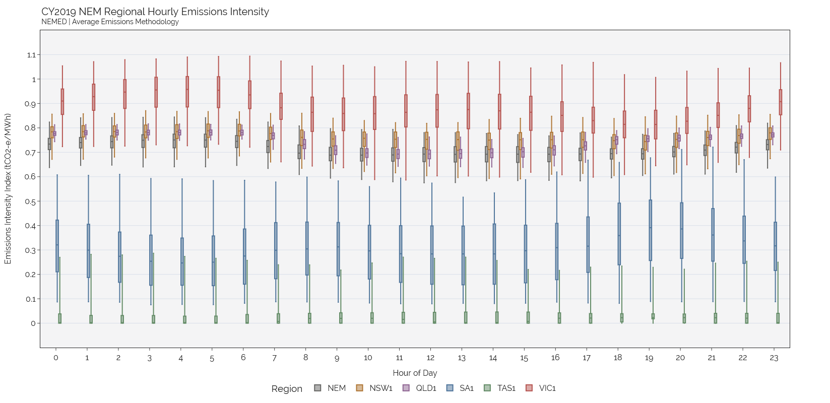
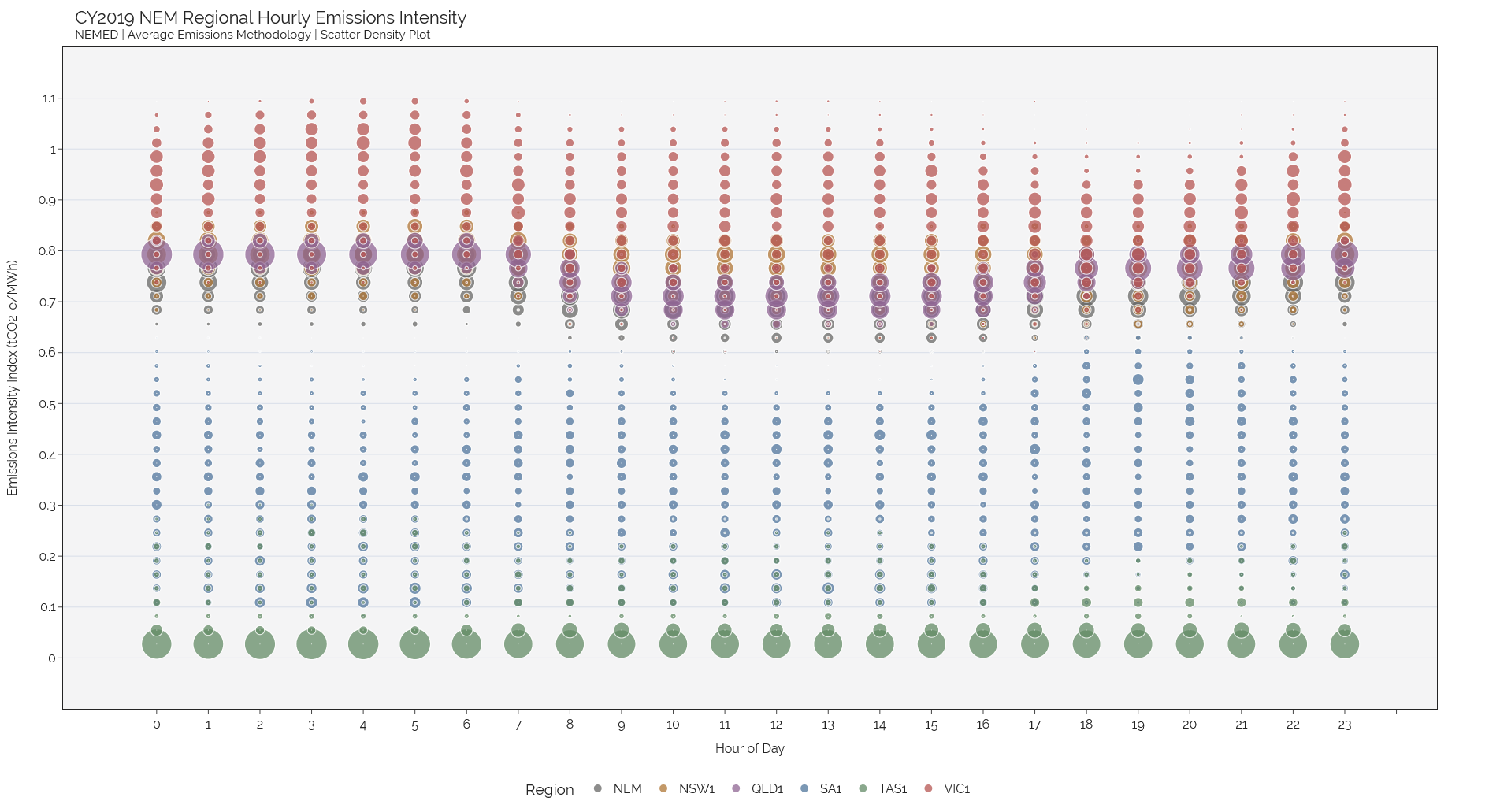
Chart 2 - Scatter Density Distribution#
Show code cell content
plt_df = co2_data.copy()
plt_df['hour'] = plt_df['TimeEnding'].dt.hour
plt_df['day'] = pd.to_datetime(dict(year=plt_df['TimeEnding'].dt.year,
                                    month=plt_df['TimeEnding'].dt.month,
                                    day=plt_df['TimeEnding'].dt.day))
plt_df['day'] = plt_df['day'].astype(str)

data = plt_df

# Time axis bins/increments
data['xbins'] = data['hour']

# Vertical axis bins/increments
bands = pd.cut(data['Intensity_Index'], 40)
data['ybands'] = bands

# For time axis, count vertical bands
bar_df = data.pivot_table(index=['Region','xbins'], columns='ybands', values='Intensity_Index', aggfunc=len, \
                          dropna=False)
bar_df.fillna(0, inplace=True)

# # Summary for bar table
bar_summary = pd.DataFrame(data.groupby(['Region', 'xbins', 'ybands']).size())
bar_summary.columns = ['count']
bar_summary.reset_index(inplace=True)

bar_summary['bin_end'] = bar_summary['xbins'].astype(str)
bar_summary['bands_end'] = [bar_summary['ybands'][i].right for i in range(len(bar_summary))]
bar_summary['bands_end'] = bar_summary['bands_end'].astype(float)

# # Plotly
fig = px.scatter(bar_summary, x="bin_end", y="bands_end", color="Region", size="count", size_max=40, \
                 color_discrete_sequence=colors, opacity=.75)
fig.update_xaxes(title="Hour of Day", tickvals=[i for i in range(0,25)], mirror=True)
fig.update_yaxes(title="Emissions Intensity Index (tCO2-e/MWh)", range=[-0.1,1.2], \
                 tickvals=[i*10**-2 for i in range(0,120,10)], mirror=True, showgrid=True)
fig.update_layout(title=f"CY2019 NEM Regional Hourly Emissions Intensity<br><sup>"+\
                         "NEMED | Average Emissions Methodology | Scatter Density Plot</sup>",
                  legend={'title':'Region','xanchor':'center','x':0.5, 'y':-0.1, 'orientation':'h'},
                  template=NORD_theme())

FONT_SIZE = 16
FONT_STYLE = "Raleway"
fonts = dict(tickfont=dict(size=FONT_SIZE, family=FONT_STYLE),
            titlefont=dict(size=FONT_SIZE, family=FONT_STYLE))
fig.update_layout(xaxis=fonts, yaxis=fonts,\
                  legend=dict(font=dict(size=FONT_SIZE, family=FONT_STYLE)),
                  title_font_family=FONT_STYLE,
                  title_font_size=22)
fig.update_annotations(font=dict(size=FONT_SIZE, family=FONT_STYLE))
fig.show()